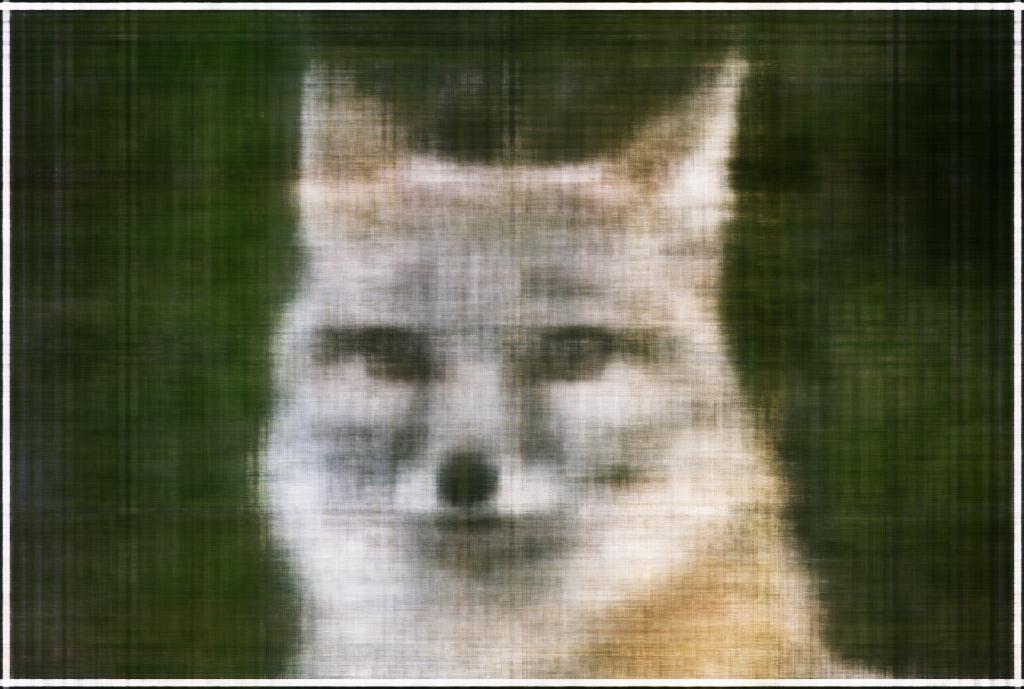
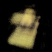
Fox

Here, we will be exploring Neural Radiance Fields (NeRF), which are used to represent a 3D space. They can accurately capture reflections and other spatial attributes, which allows them to still show the physical aspects of something while also providing new views.
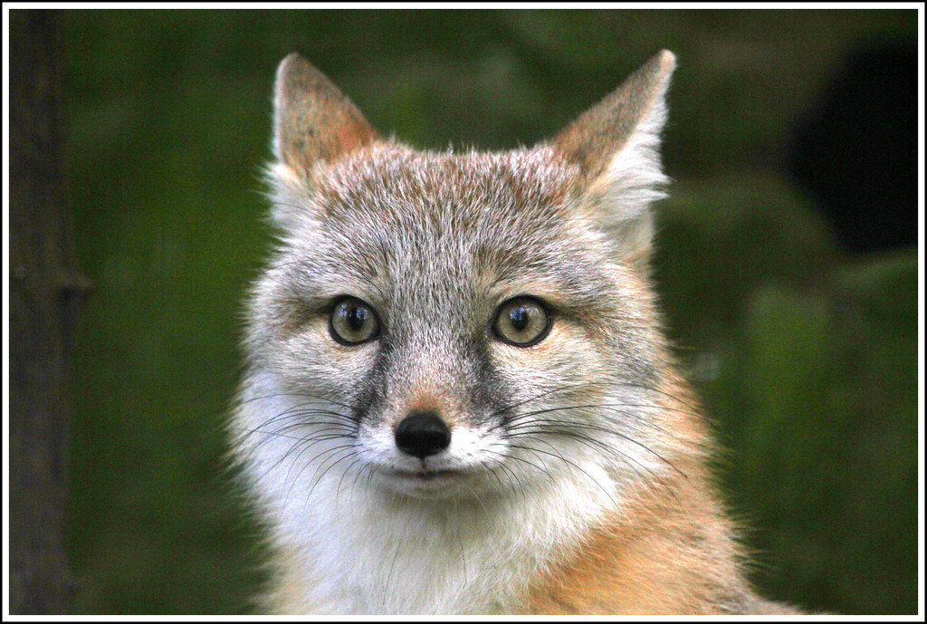
In this part, we will create a neural field to learn the images.
In this step, we implement the MLP, which is the foundation of the neural field. It is a four layered structure, going from an x that is 2D to an rgb that is 3D. We also create a sinusoidal positional encoder to expand the input's dimensionality, thereby helping the model learn more complexity.
Now we create a dataloader to take the image, and then randomly sample and return pixels for every iteration in the training cycle.
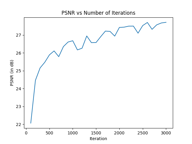
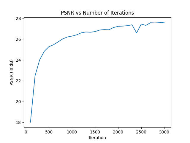
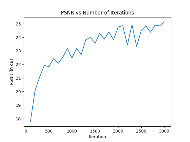
The next part is the loss function, the optimizer, and the metric used to evaluate. We used MSE for the loss function, while also using the Adam optimizer. The metric is PSNR, or peak signal-to-noise ratio, calculated through the ratio of max power a signal and the max power of corrupting noise.
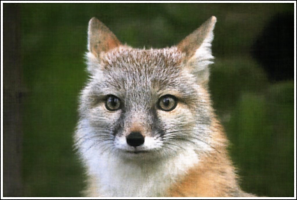
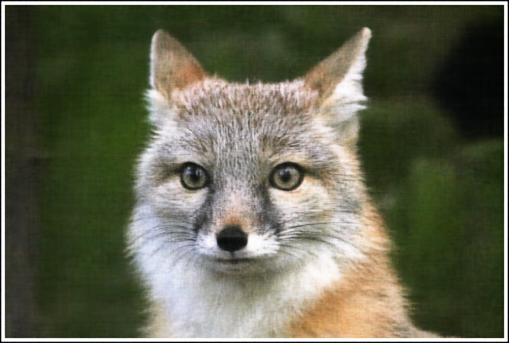
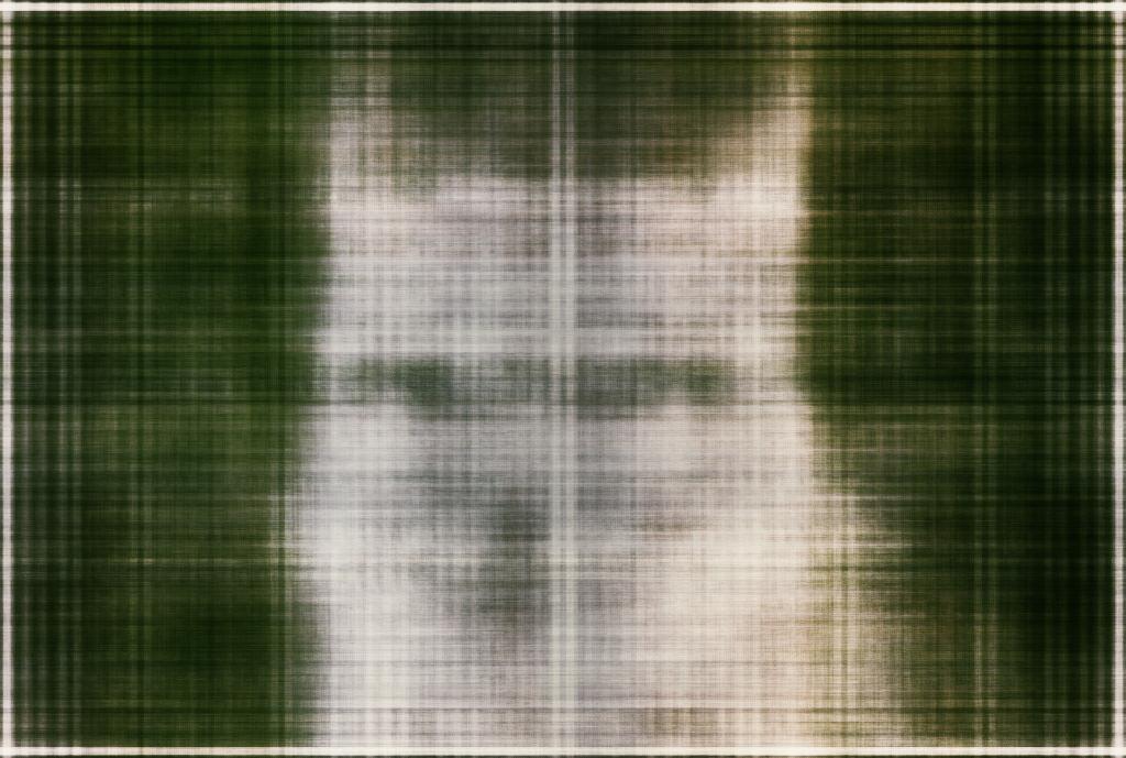
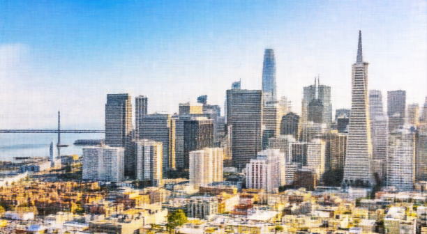
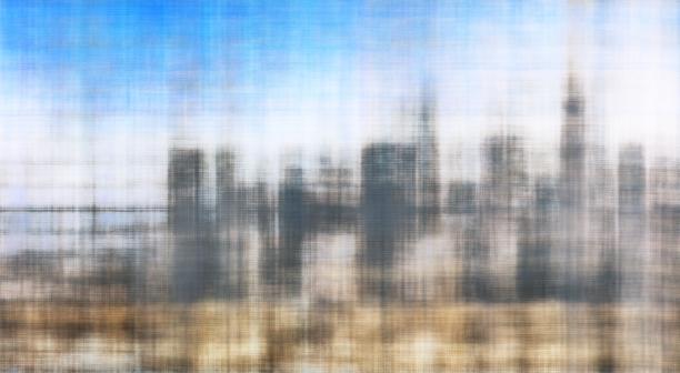
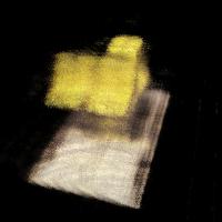
This is the training, where I created two models for the fox image, while also creating a model for san francisco, creating a gif for each to show how the iterations function. The batch size was 10,000.

Here, we will be implementing the Neural Radiance Fields (NeRF).
Here, we create rays from cameras. We implemented the generation of rays using c2w matrices and focal length, first using a transform function to convert into world coordinates, and then implementing both pixel to camera and pixel to ray, both of which involved transforming the pixel into either camera coordinates or ray origins.
Here, we sampled from the rays, sampling 64 samples along the ray, and then offsetting by 0.5 pixels.
Here, we implemented a dataloader, which takes in images, c2w matrix, and the K matrix, to compute the rays for each image. Then, sampled a batch of rays, an example of which is below:

Here, we implemented the NeRF model, which has an MLP that takes in a ray origin, direction, and depth, and outputs color and density values. We used positional encoding again, and then had two branches of MLP dealing with color and density. We trained this model using a learning rate of 1e-3 and a batch size of 10000.
Here, we implemented volume rendering, which is basically a weighted average based on the probability of the ray not terminating before the current depth.
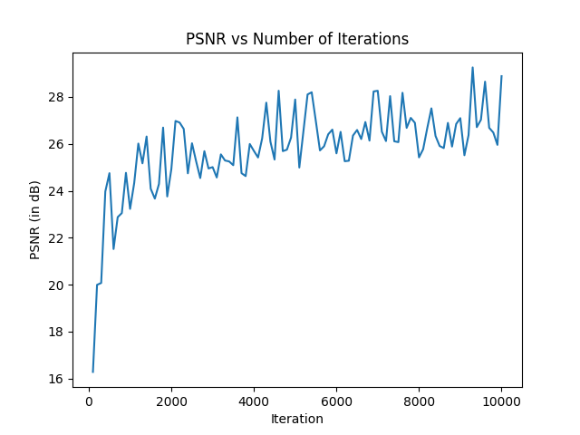
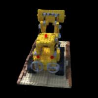
Here, we finally were able to train the model, using the adam optimizer and a learning rate of 1e-3 and a batch size of 10000. We initially trained with 3000 iterations, but eventually trained with 10000 iterations for the final render, taking about 30 minutes to run.
Here we implemented depth rendering, where we accumulated depth instead of color in the volume rendering algorithm, the result of which is below: