Today we will be investigating morphing, starting with part a where we explore diffusion, and part b where we implement diffusion models.
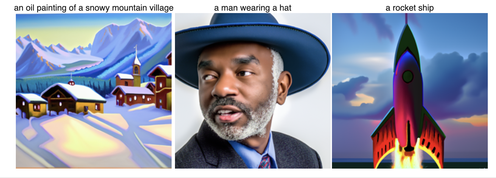
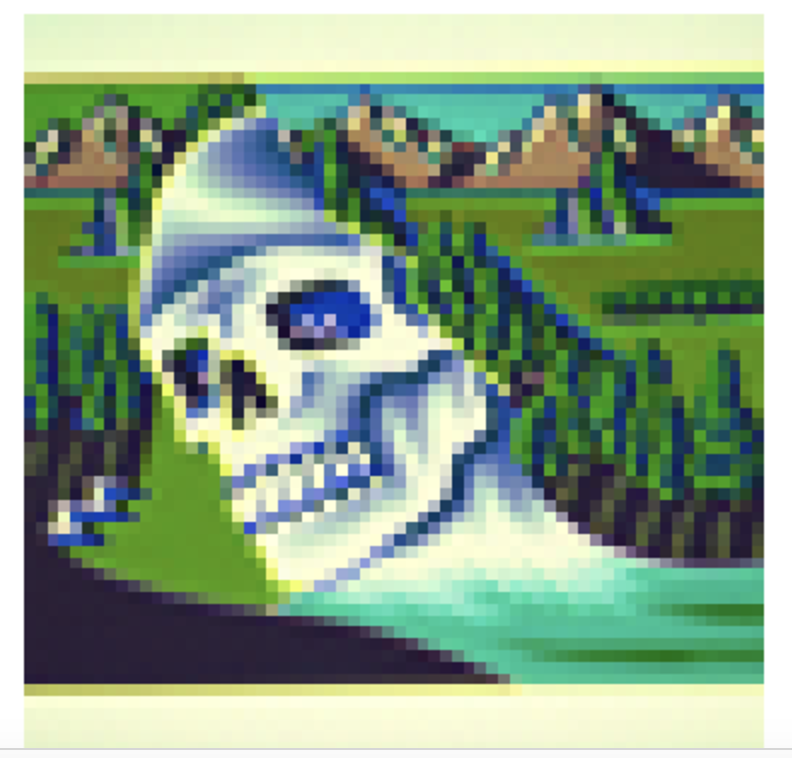
I am using a random seed of 30, and below are the caption output pairs for the model for the three text prompts provided.

Now we are implementing the forward process, which involves taking a clean image and adding noise to it. Basically, given a clean image, we can get a noisy image at time step t by sampling from a Gaussian. The test images below are at 250, 500, and 750 noise levels.

This next part is classical denoising, where I remove the noise from the images from the previous part using Gaussian blur filtering. There are not great results from this.
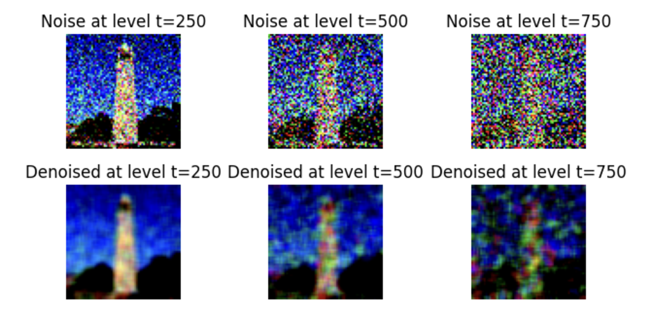
This next part is one step denoising, where we use a pre-trained UNet to recover Gaussian noise from the image, which means that we can try to recover the image using what the model thinks is Gaussian noise. We use the prompt "a high quality photo".
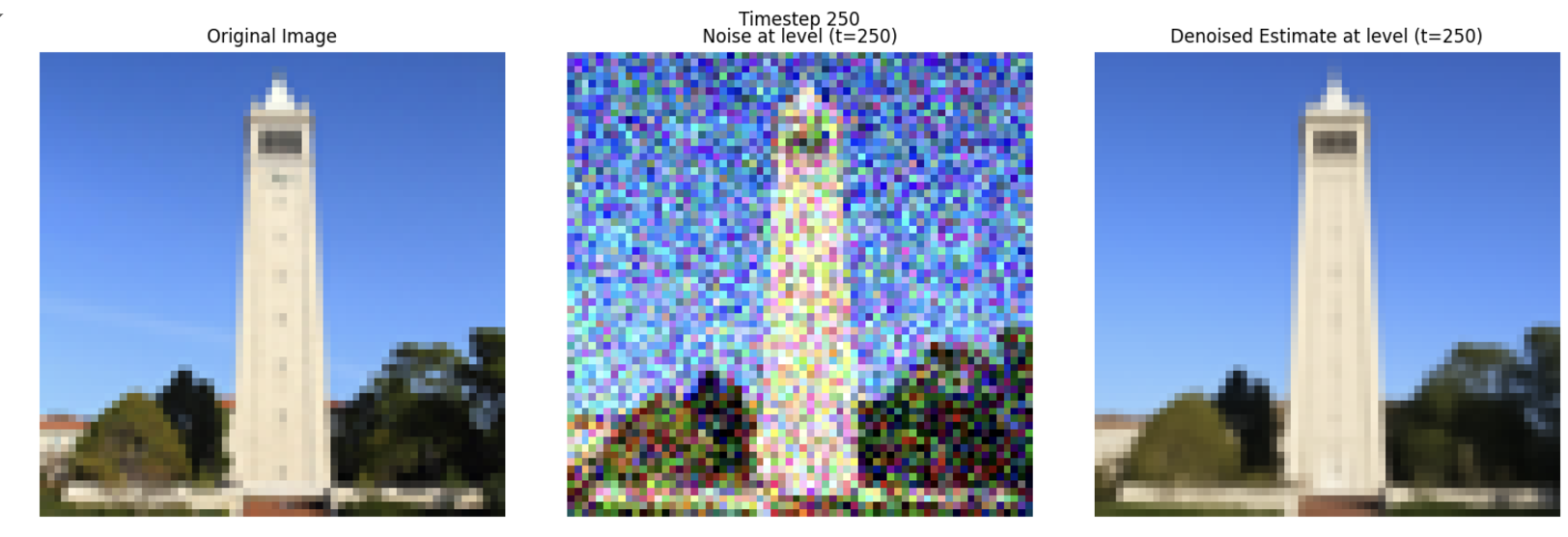
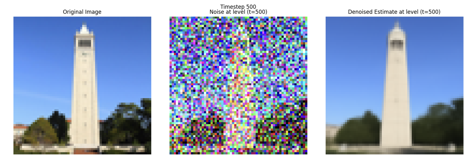
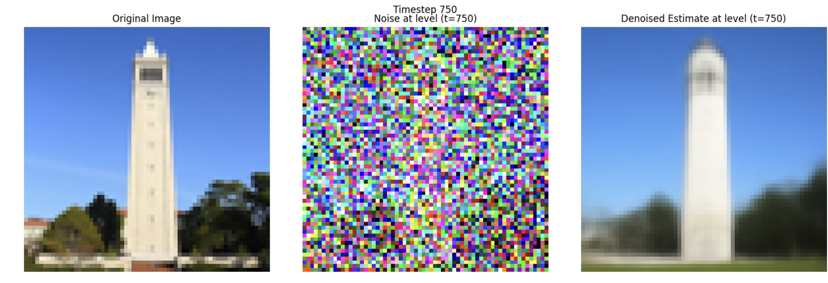
In this part, I implement iterative denoising, where I use strided timesteps to "skip" steps in the iterative denoising process, which allows us to properly denoise and get a pretty clean image. The first set of images is the iterative denoising every five steps.
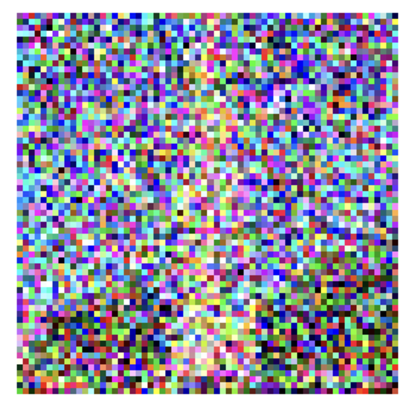
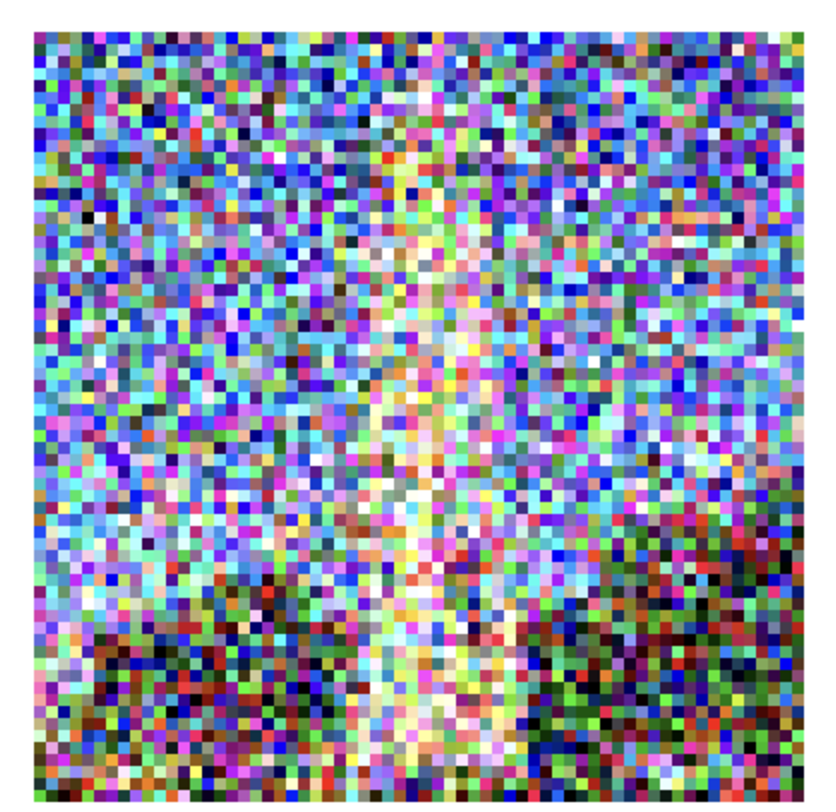
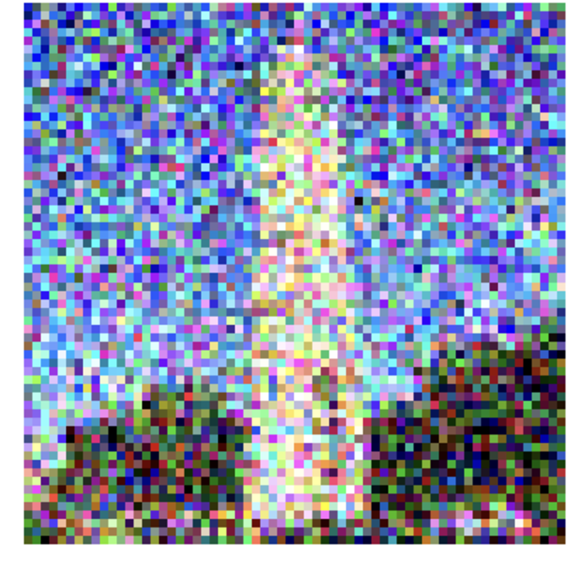
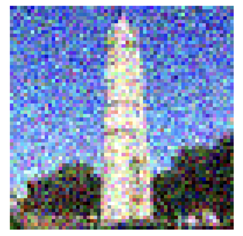
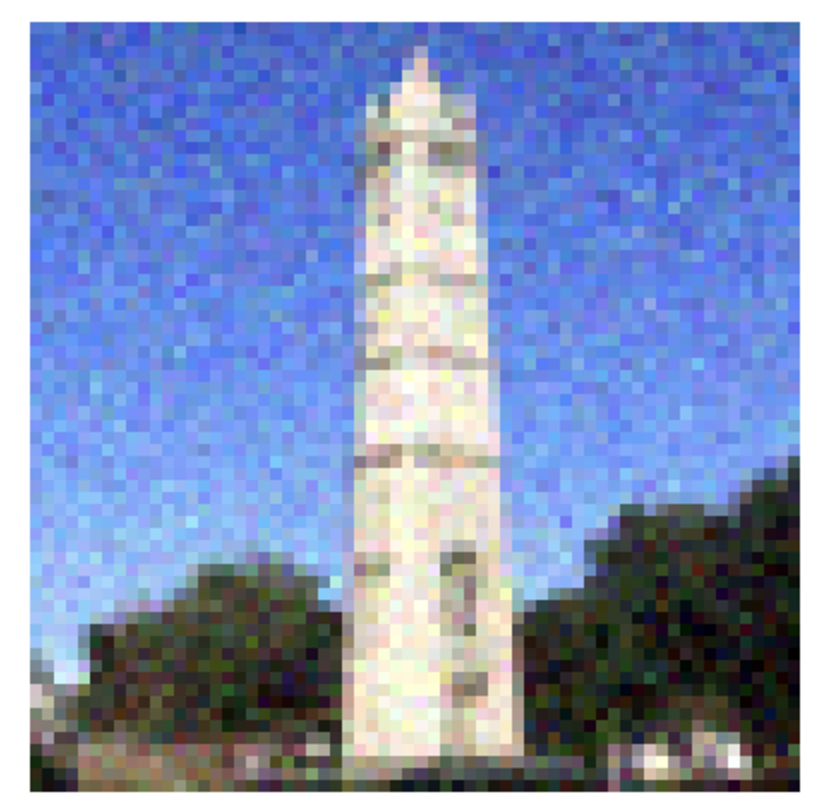
From left to right, original image, noisy image, clean image using iterative denoising, clean image using one step denoising, and clean image using gaussian blur.

Here, we are now doing diffusion model sampling, where we use a diffusion model to sample an image. We are generating images from scratch using the prompt "a high quality photo", starting with random noise.

Here, we are doing Classifier Free Guidance to improve the image quality that came from the previous section. We basically use the conditioned and unconditioned noise estimate on a text prompt to better compute a noise estimate and therefore denoise better.

Here, we are going to take an original image, then force it back to the original image manifold after adding some noise, a process whose results are shown below.

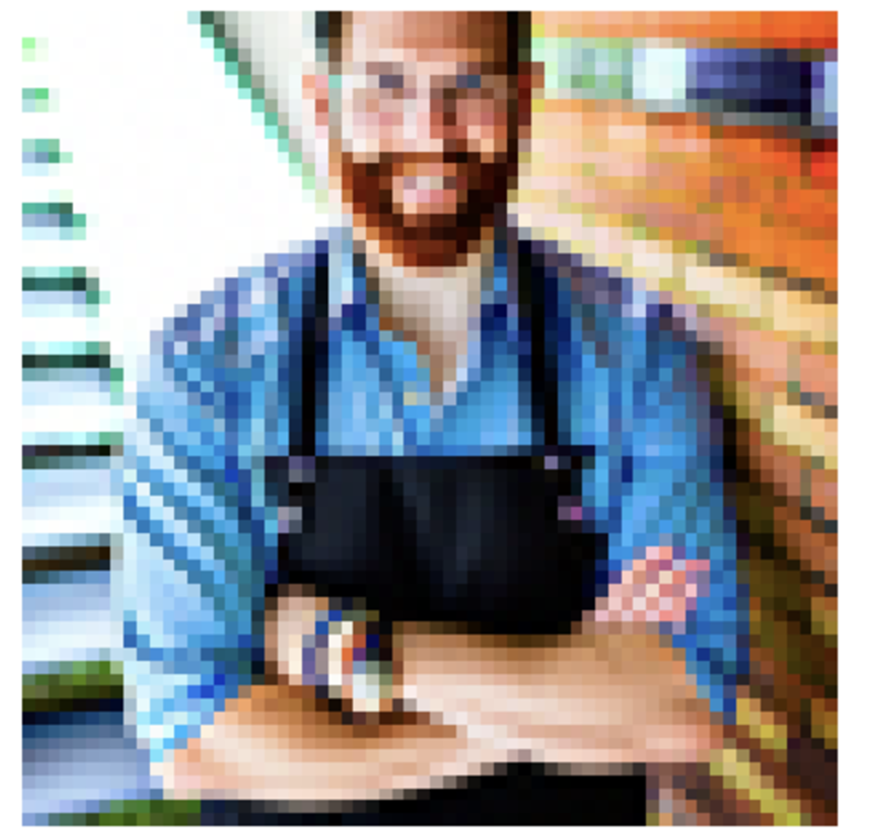
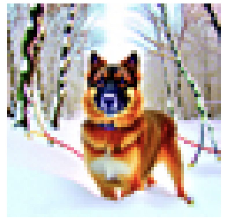
Here, we are going to do the same thing, except with 1 web image, and 2 hand-drawn images below (original images on the left).
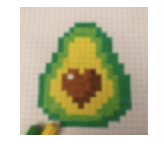

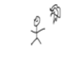


Here, we are going to work with inpainting, where we implement inpainting, using a binary mask.
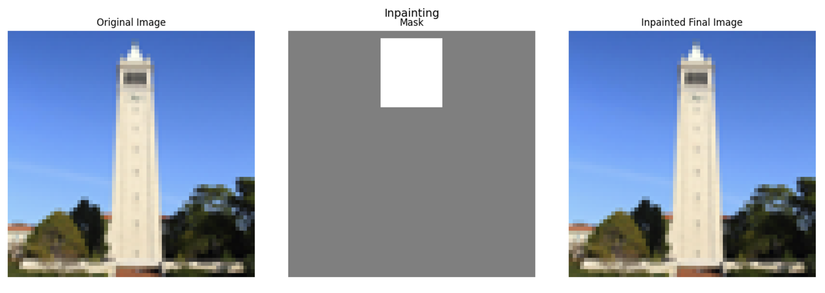
Here, we are going to use the same inpainting techniques, but we are also going to take into account a different prompt, in this case "a rocket ship".

Here, we are going to use the same principle we used, except create a visual anagram, where you can see one image when the canvas is oriented one way, and then you can see a second image when the canvas is oriented the other way.
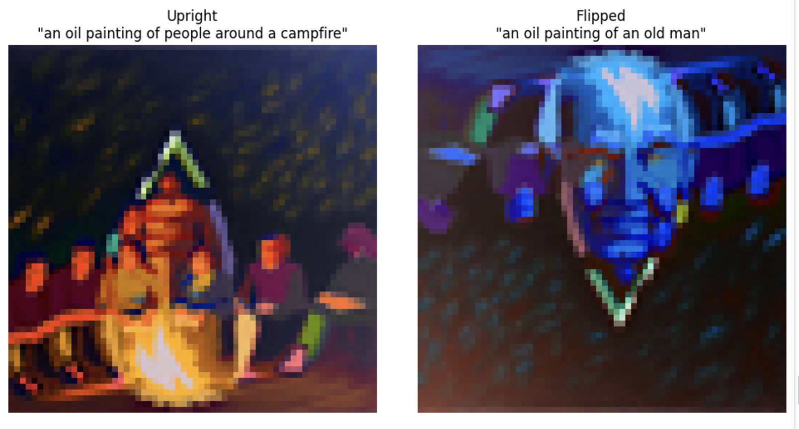
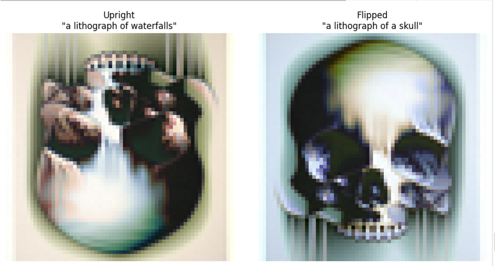
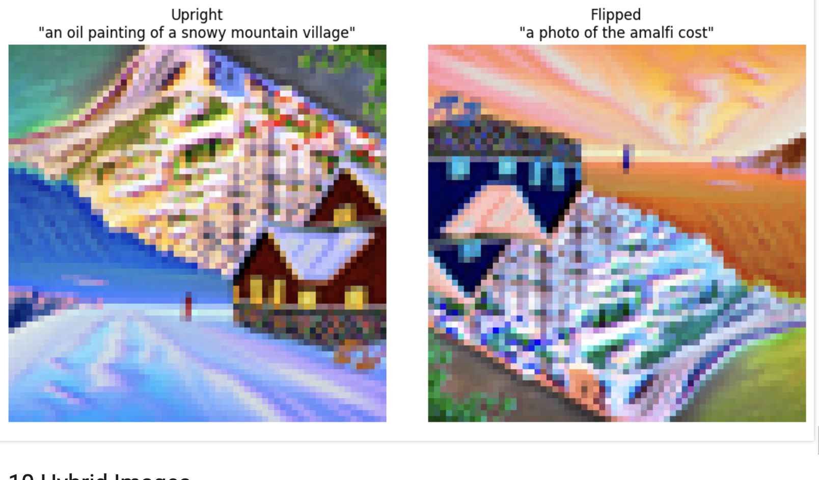
Here, we are going to create hybrid images using factorized diffusion. We are creating a lowpass and highpass again, and this allows us to see an image when close, and an image when far.
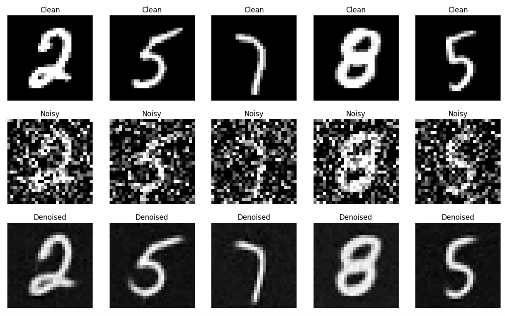
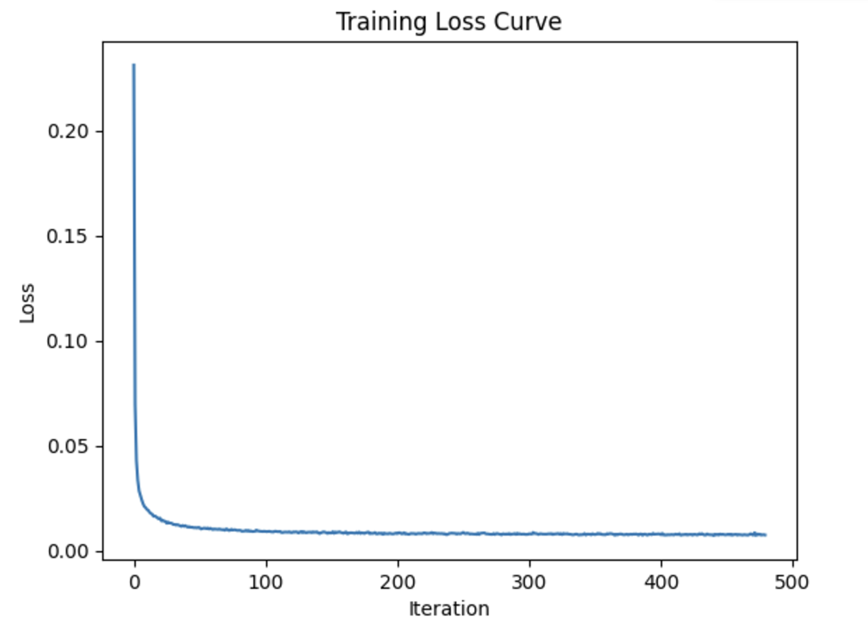
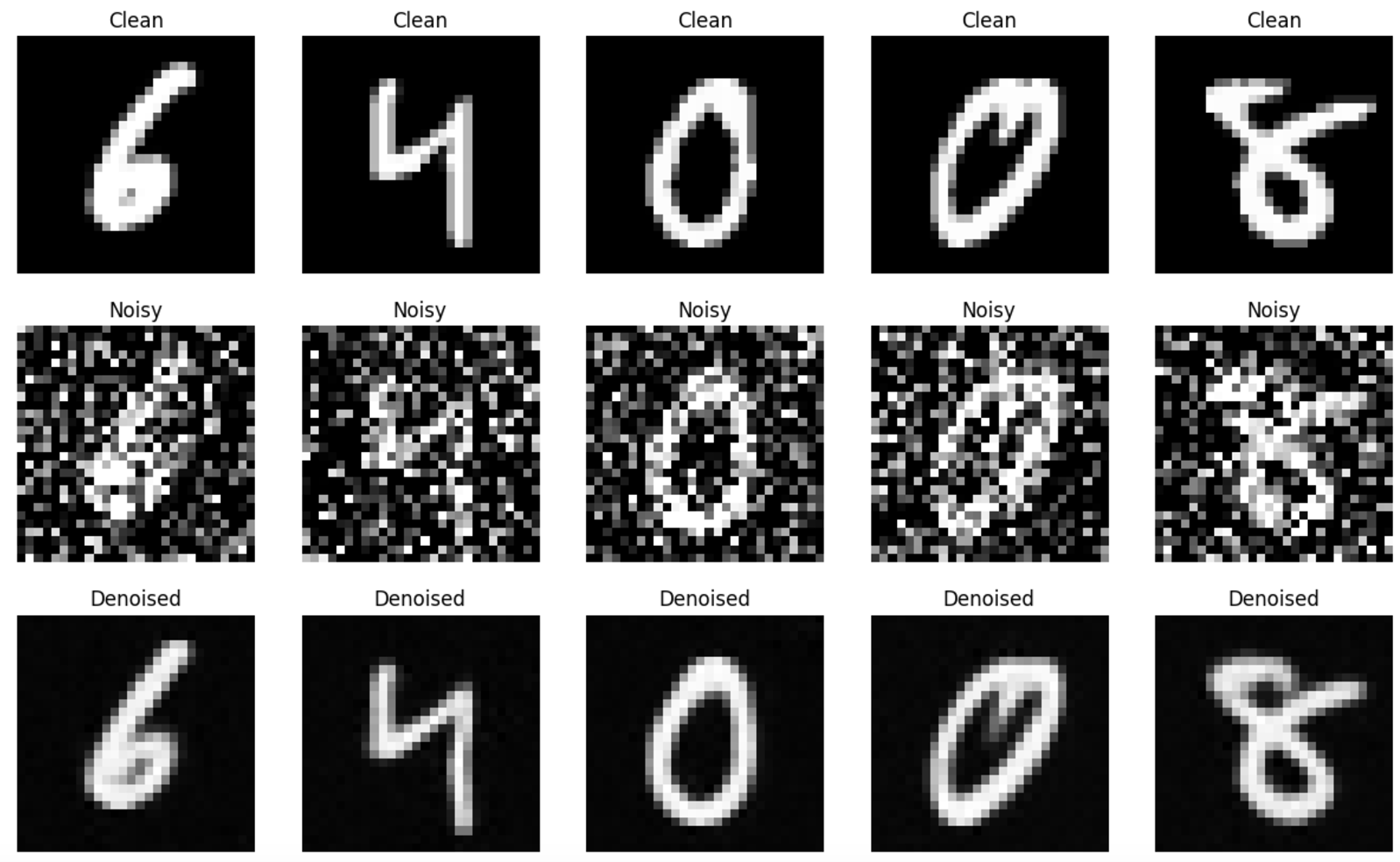
Here, we are starting with training a simple UNET denoiser, using a sigma value of 0.5 for noise level. We are optimizing over an L2 loss, and we train the denoiser over noisy + clean pairs. Below (from top to bottom) is a visualization of the noising process, training plot of loss, sample results on the test set, and sample results on the test set for all the sigma values.

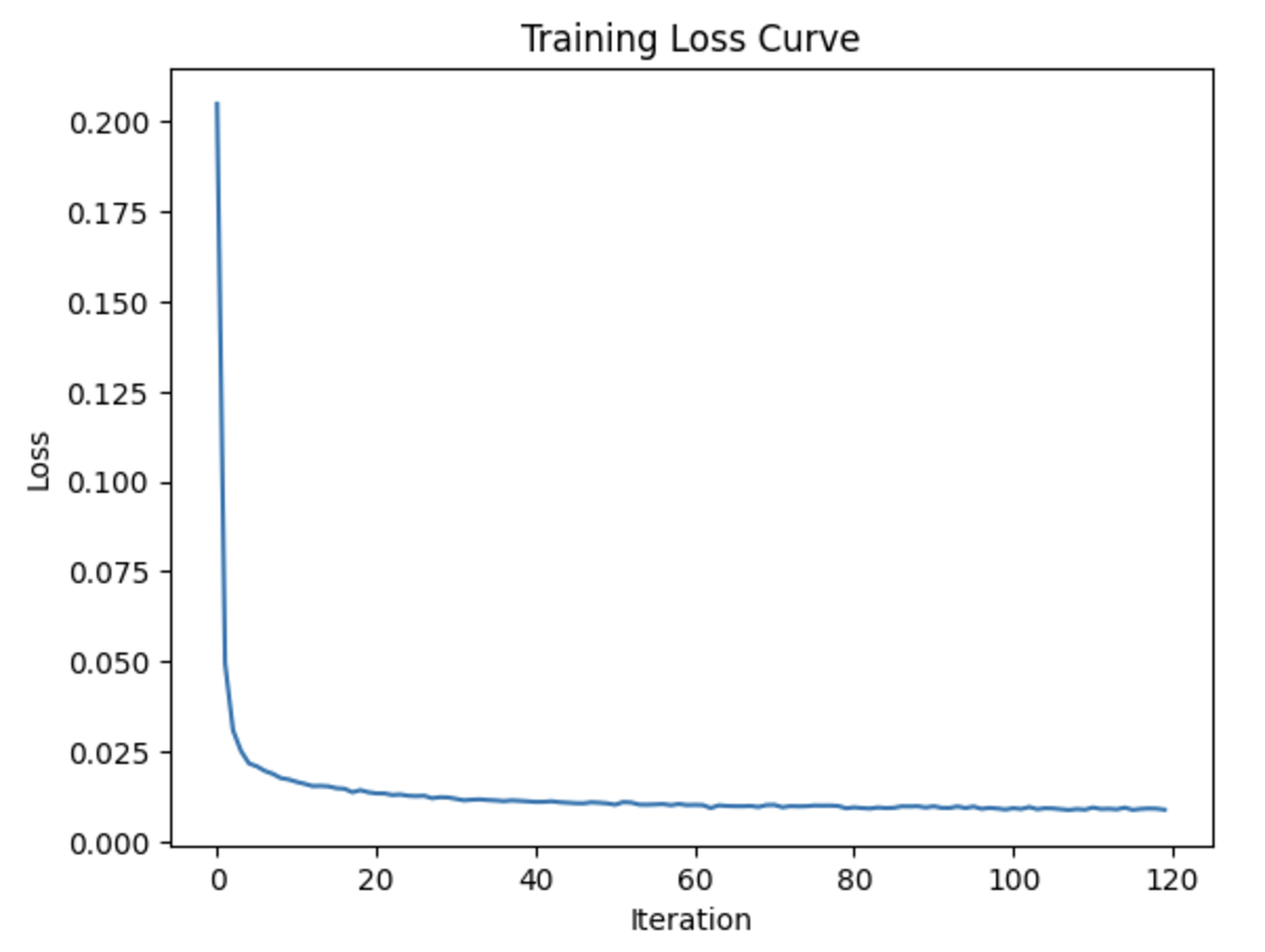
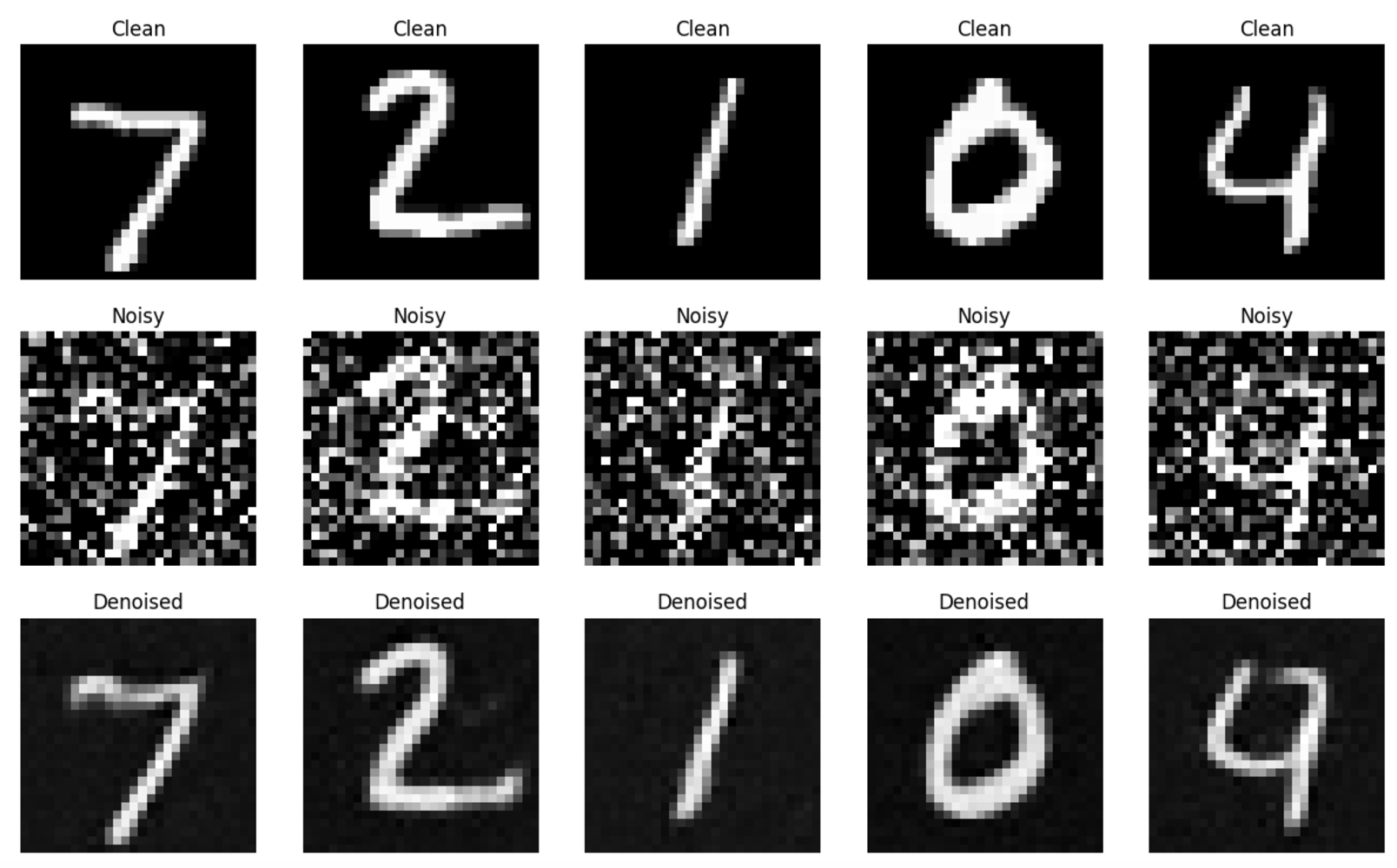

Here, we add time-conditioning to the UNet, starting with predicting added noise to the image. Then, we add a scalar t into the UNet to condition it, using an FCBlock. Now, using a random t and image, we train the UNet to predict the noise. Then, we sample from the UNet. Below (from the top down), we have a sample from the 5th epoch, and then the training curve for the entire training process, and then the sample from the 20th epoch.
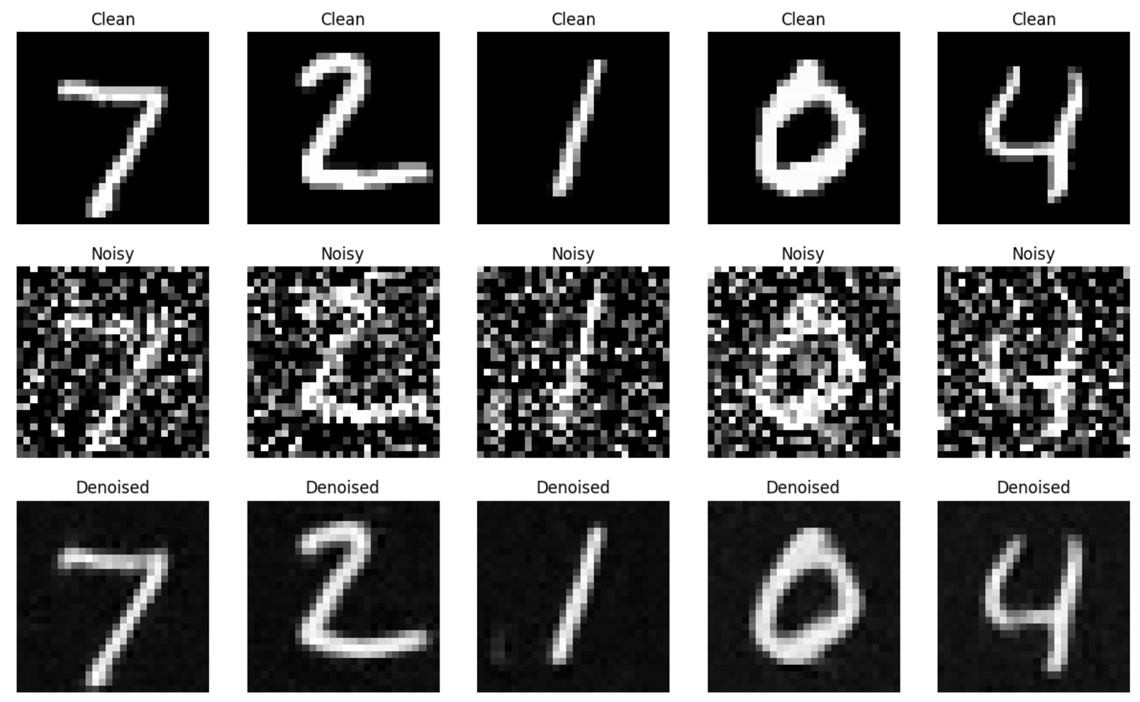
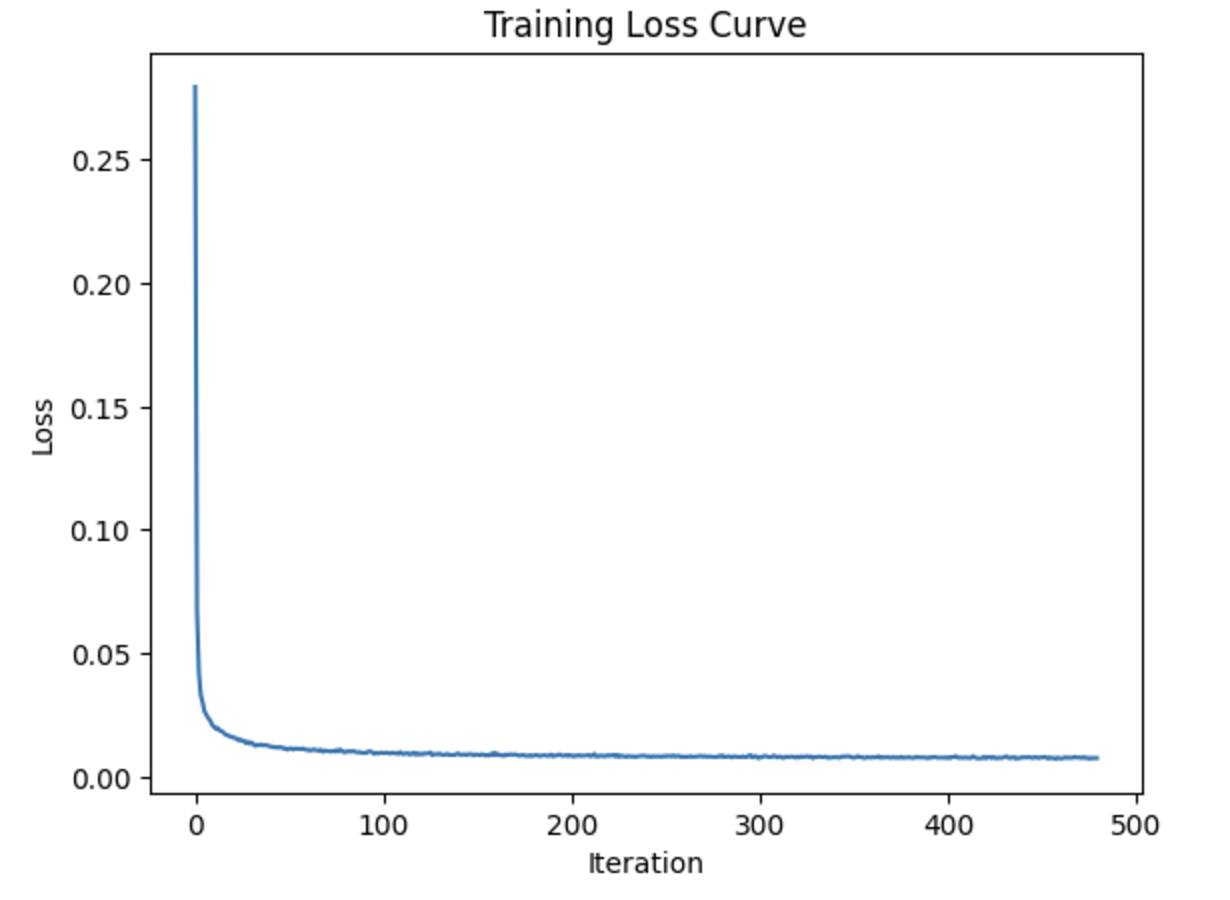
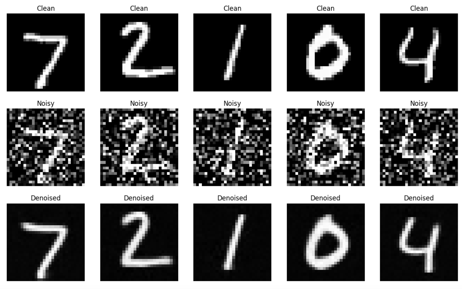
Here, we add class-conditioning to the UNet, where we want to gain better control for image generation. So, we condition the UNet on the digit 0-9, using a one-hot vector. Below (from the top down), we have a sample from the 5th epoch, and then the training curve for the entire training process, and then the sample from the 20th epoch.
